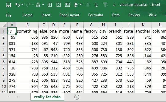
VLOOKUP that fat table with ease [3 quick tips] -

Time for some good, old fashioned VLOOKUP love. Let’s say you are writing VLOOKUP()s to get data from an unusually fat table, ie one with heaps of columns. You want to get to lookup ID in first column and get thingamajig in what is that column number. Well, better get counting from 1 and after 19 seconds and lots of squinting you arrive at column number 53 – which has thingamajig.

If this sounds like your VLOOKUP routine, check out these three amazingly simple tips to save some time and effort with your lookups.

#1 Switch to R1C1 view

This is a quick and easy fix. Head to File > Options > Formulas and enable R1C1 reference style. This will tell you what each column is in number format. Problem solved.

Of course, this also means all your formula references will be turned in to R1C1 style. But once you disable the R1C1 reference style in Formula Options, your VLOOKUP will be back to A1 style.

#2 Use Tables

While the R1C1 view can quickly tell you what each column is in numbers, it won’t work if your data starts from 17th column or something like that. A better option is to turn your raw data in to tabular format using Insert > Table. Give this table a name from Design ribbon, like mydata. This way, you can use simpler lookup formulas.

Original VLOOKUP: =VLOOKUP(something, data!$A$2:$BK$123, 53,false)

VLOOKUP using tables: =VLOOKUP(something, mydata, 53,false)

But we still have to figure out the column for thingamajig. Simple, we use MATCH() formula inside VLOOKUP, like this:

VLOOKUP using tables & MATCH(): =VLOOKUP(something, mydata, MATCH("thingamajig", mydata[#Headers], 0), false)

That is right, you can access table headers using the #Headers keyword and get position of any header.

#3 Use INDEX + MATCH

This will make the problem altogether irrelevant. Simply use INDEX and MATCH formulas to get the result you need, like this:

=INDEX(mydata[thingamajig], MATCH($C$3,mydata[ID],0))

Now, you don’t care if thingamajig is 53rd column or 217th column and if ID is at the start or somewhere else. It works all the same.

For more about using INDEX in your formulas, check out this beautiful tutorial.

Here is a summary of all formula techniques

Normal Lookup [help]
Formula	`=VLOOKUP(something,'really fat data'!$A$2:$BK$123,53,FALSE)`
Comments	You need to know which column (53) has the data you need. Either count manually or enable R1C1 style to quickly to know.

Using Tables [help]
Formula	`=VLOOKUP(something,mydata,53,FALSE)`
Comments	Create a table for your source data (using CTRL+T) and give it a name. Use the name in your formulas. You still need to know column number.

Using Tables + MATCH()
Formula	`=VLOOKUP(something,mydata, MATCH("thingamajig",mydata[#Headers],0),FALSE)`
Comments	Use MATCH() to find out which column header has the value you want to lookup.

Using INDEX + MATCH [help]
Formula	`=INDEX(mydata[thingamajig], MATCH($C$3,mydata[ID],0))`
Comments	Now, you don’t even need to know where everything is. Just lookup the value in ID column and get corresponding value from thingamajig column. Done