Recently, Paul, a reader, of the Chandoo Blog Post: Colors-in-excel-chart-labels-trick asked a question:
“Hi Chandoo,
Is it possible to change the background label color on chart depending on the value? ”
I answered with a general “Yes” and offered two solutions
1. Using CF to color the background cells behind the chart
2. A VBA Solution to change the chart colors
This post will examine how to implement each method:
I have attached sample files which includes both examples Excel 2007-13 Sample or Excel 97-2003 Sample
You can follow along in this file before attempting it on your own data.
Using Conditional Formatting to Color the background cells
In the sample file goto the CF Technique worksheet
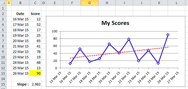
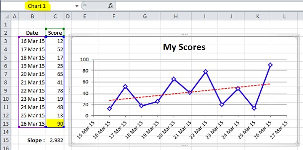
In CF Technique worksheet you will see a set of data with dates and Scores for each date
Below the main table is a calculation of the slope of the line of best fit through the data
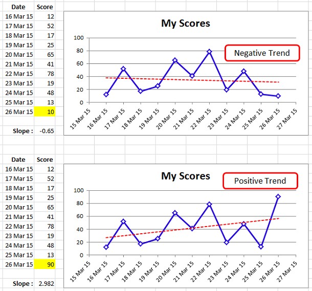
This shows either a positive number when the data is trending upwards or a negative number when it is trending downwards
For the purpose of this we can simply change the yellow cell C13 from 90 to 10 to change the slope from a Positive to a Negative value
Next to the chart is a simple X-Y Chart showing the Scores vs the Date (Blue) and a Line of best fit (Dashed Red)
The chart is exactly covering the range E3:L15, this is achieved by placing the chart roughly in position and then holding the Alt Button whilst dragging the corners or edges of the chart.
Note: The use of Alt forces Excel to Snap the object onto the cell edges and lock it there, so that when the column width or row height changes, the Chart will resize with it.
Next we set the colors of the Chart Area and Plot Area to Transparent (No Color)
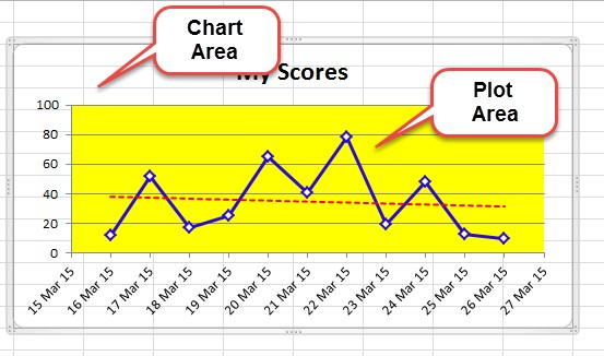
The Chart area is the Background area of the chart, White in the following example
The Chart area is the Background area of the chart, Yellow in the following example
We can see that the chart area has no color in the above picture as we can see the Grid Lines through the Chart Area.
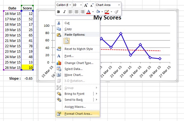
Format the Chart Area
Select the Chart
Right Click in the Chart Area,
Format Chart Area
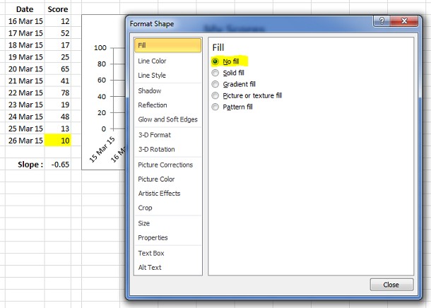
Click on the Fill Tab and set the Fill to No Fill
Format the Plot Area
With the chart selected, Right Click in the Plot Area,
Format Plot Area
Click on the Fill Tab and set the Fill to No Fill
Click outside the chart
Apply a Conditional Formatting to the Range behind the Chart
Select the range E3:L15 (You won’t be able to use a mouse) or drag the chart out of the way first.
Goto Conditional Formatting Tab
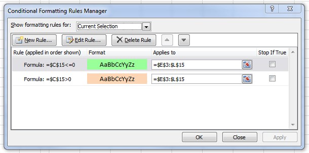
New Rule
Use a formula to determine which cells to format
Enter the formula: =$C$15>0
Select the Format Button and select a Light Redish Color
Ok
Goto Conditional Formatting Tab
New Rule
Use a formula to determine which cells to format
Enter the formula: =$C$15<=0
Select the Format Button and select a Light Greenish Color
Ok
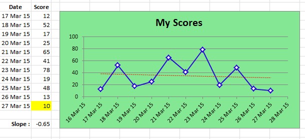
Now change the value of C15 from 90 to 10
The chart should change as per the below image:
Advantages:
- Doesn’t require VBA (VBA not permitted on some corporate systems)
- Simple to setup for those unfamiliar with VBA
Disadvantages:
- The Chart is locked to the cells and can’t be moved moved independently of the background cells
- More difficult to implement multiple color scenarios
- Harder to permit independent changes to the Chart and Plot areas
Using VBA to directly change the color of the Chart Chart Area
In the sample file goto the VBA Technique worksheet
You will see the same set of data with dates and Scores for each date
Select the Chart and notice that the Chart is called “Chart 1″
Goto VBA, Press Alt+F11
Double click on the VBA Technique code module
Copy and paste the following code into the module
Private Sub Worksheet_Calculate()

Dim myColor As Long
Dim myChart As String

Application.EnableEvents = False

If ActiveSheet.Name <> "VBA Technique" Then Exit Sub

myChart = "Chart 1"

If [c15] <> [OldSlope] Then

  If [c15] > 0 Then
    myColor = RGB(250, 190, 145) 'Apricot
  Else
    myColor = RGB(135, 235, 145) 'Pale Green
  End If

  ActiveSheet.ChartObjects(myChart).Activate
  ' Color the Chart Area
  With ActiveSheet.Shapes(myChart).Fill
    .Visible = msoTrue
    .ForeColor.RGB = myColor
    .Transparency = 0
    .Solid
  End With

  ' Color the Plot Area
  ActiveChart.PlotArea.Select
  With Selection.Format.Fill
    .Visible = msoTrue
    .ForeColor.RGB = myColor
    .Transparency = 0
    .Solid
  End With

  ActiveWorkbook.Names.Add Name:="OldSlope", RefersToR1C1:="=" + CStr(Cells(15, 3).Value)
End If

Application.EnableEvents = True
Range("C17").Select

End Sub
Return to the Excel worksheet
Now change the value of C15 from 90 to 10
Advantages:
- Allows the Chart to be moved independently of the background cells
- Allows a much simpler implementation of multiple color scenarios
- Allows independent changes to the Chart and Plot areas as well as other Chart Elements
Disadvantages:
- Requires VBA (not permitted on some corporate systems)
Other Chart Conditional Formatting Posts
You may also be interested in the following Chart Formatting posts:
http://chandoo.org/wp/2011/08/19/selective-chart-axis-formating/
http://chandoo.org/wp/2011/08/22/custom-chart-axis-formating-part-2/
Closing
What do you think of these techniques?
Let us know in the comments below.

