We all know pivot table functionality is a powerful & useful feature. But it comes with some quirks. For example, we cant insert a blank row or column inside pivot tables.
So today let me share a few ideas on how you can insert a blank column.
But first let’s try inserting a column
Imagine you are looking at a pivot table like this.
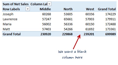
And you want to insert a column or row. Go ahead and try it. Here is what happens.
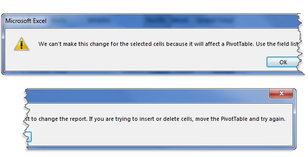
- Excel gets mad thinking you are attempting anarchy and throws a stern, but very long & confusing warning message.
In fact the error message is so long, I can’t even fit it in one image on this blog. Here it goes, verbatim.
So how DO we insert a column in the pivot
The answer is simple.
Don’t
Don’t bother inserting the columns in actual pivot table. Instead, follow this approach.
- Select any cell in the pivot
- Press Ctrl+Shift+8 – This selects the entire pivot
- Copy it by pressing CTRL+C
- Go to a new worksheet
- Paste as references – ALT+CTRL+V and L
- Select any cells containing 0 and press DELETE key
- Now, go ahead and insert any number of columns & rows in this new worksheet
- When your pivot changes (either due to refresh or new data), the copy worksheet changes too
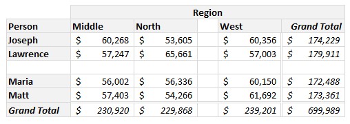
- Bonus: You can format the new worksheet cells any way you want. It just works.
Here is an example of what you can do.
But I want to insert a column in my pivot!!!
Okay, clearly you have a case of OCDIS (Obsessive Column Deletion / Insertion Syndrome).
Here is one way to technically insert a column inside the pivot table.
Before understanding the process, let’s pause and ask, “why do you want to insert a column?”
Here are few possible reasons.
- Cosmetic / formatting reasons. A blank column makes things easy to read
- To add commentary / notes / extra data
- To perform intermediate calculations on the data
If your answer is 1, the above approach (copying pivot and pasting as references) gives you most control over the layout and formatting. Go for it.
If your answer is 2, again above approach is still good.
If your answer is 3, you can use calculated item / fields is your best option.
If your answer is 3 & you are using Excel 2013 (or power pivot), you can use either Sets feature or MDX formulas to mimic blank rows. Unfortunately, I can’t explain this because squirrels know more MDX than me.
Let’s say you want to calculate certain percentage or similar…
Okay, so want to calculate North / West % in below pivot.
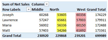
In this case, you can use calculated items feature of pivot table like this.
- Select any region name in the column labels are of pivot
- Go to Home > Insert > Calculated Item
- Give your calculated item a name like “North by West %”
- Write the formula =North / West
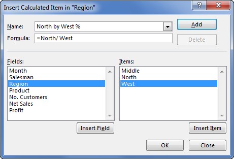
- Click ok
- This new column will added to your pivot, like this:
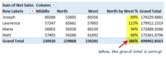
As you can see, it works fine until we hit the grand total row. There our North / West % should be 96%. Instead it reads 386%. Clearly a number calculated by my 6 year old son.
Why is the total wrong? Because, pivot table grand totals are a simple sum of all the above values. So Excel went ahead and added up the four percentages.
How to fix this? One simple options is to turn off the grand totals. Note that even row level grand totals are off as the % was added to actual values.
If you must see the grand totals, then your best bet is to use Power Pivot. It allows you to define formulas (using DAX) and create powerful pivot tables.
So no easy way to insert columns then?
It took us a few minutes to get here, but that is the answer. There is no simple work around to this problem. Instead, here is a 4 step process you should follow.
- Take a few deep breaths
- Insert your favorite expletive in this sentence “______ pivot tables” and shout it.
- Use Power Pivot
- If Power Pivot cant be used, copy the pivot as references and manipulate the layout as you wish.
Happy pivoting.


