One of our readers emailed this question recently,
I like the conditional formatting icons. I am trying to present some business data where going down is good. How do I get a green colored down arrow icon?
Essentially, Ms. CanIGetItInGreen wants this:
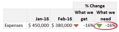
Unfortunately, Excel’s conditional formatting icons are not customizable. So we can’t get the green down arrows without some sneak. And sneak we shall.
Green color down arrows, red color up arrows – Tutorial
- Let’s say you have calculated a number (percentage change for ex.) in cell F4.
- In adjacent cell, write =IF(F4>0,”p”,”q”) This will return p if the value is positive and q otherwise
- Now change the cell font to wingdings 3. This will change the values p & q to up & down arrow symbols.

- Change font color to green.
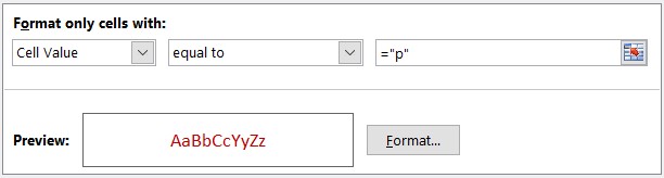
- While keeping the cell selected, go Home > Conditional Formatting > New Rule
- Set up a rule to color the cell value in red when it is p.
- If you wish to see the % value, keep the adjacent cell (F4), else hide it.
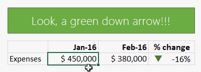
Here is the final thing:
Learn awesome conditional formatting tricks
Conditional formatting is one of my most favorite areas of Excel. It has a ton of potential and offers a lot of creative freedom. Check out below tutorials to power up your conditional formatting mojo.
- Monthly planner template with formulas & conditional formatting
- How countries spend their money – conditional formatting chart
- Dashboard best practice: Highlight user selection with conditional formatting
- Data entry: Cleaner input dates with conditional formatting
- Fun: Modeling tiles in a room using conditional formatting
How would you turn the arrow green?
Would you use the above approach or something else? Please share your ideas in the comments section.


