Unpivot data quickly with Power Query [tutorial] -

Power Query (Get & Transform data in Excel 2016) is a must have tool, if you wrangle with data every day. Here is a quick introduction, in case you are new.

Let’s learn how to use Power Query to unpivot data.

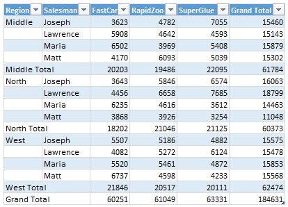
Essentially, we are trying to go from left to right in this picture.

Doing something like this thru either formulas or VBA can be very complex. But Power Query can get you unpivoted data in just a few clicks. Sounds interesting? Read on.

Tutorial: Unpivot data using Power Query

Step 1: Set up your pivoted data as a table

If you want Power Query to work with data in Excel, it must be in table form. So select any cell in the pivoted data and press CTRL+T to turn it in to a table.

At this stage, we get this:

Step 2: Load table data in to Power Query

While keeping the selection inside pivot data, go to Power Query ribbon (or Get & Transform area of Excel 2016 data ribbon) and click on “from Table” button.

This will take your table data and load it in to a new query in Power Query. It looks like this:

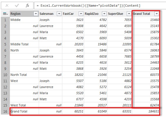
Step 3: Get rid of grand totals

When unpivoting data, we don’t need the grand totals. To remove them,

Select the grand total column
Click on “Remove Columns” button in query editor (Power Query window)
Click on “Remove Rows” button, select remove bottom rows option.
Enter the number of rows as 1

At this stage, grand total column & row are gone. We end up with this:

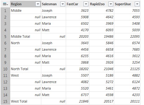
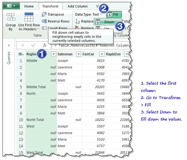
Step 4: Fill down the missing region names

If your pivot table has null / blank values in the first column, you can fill them with values from above cells using the Fill option of query editor. Select the Region column and click on the Fill button from transform ribbon. See this demo:

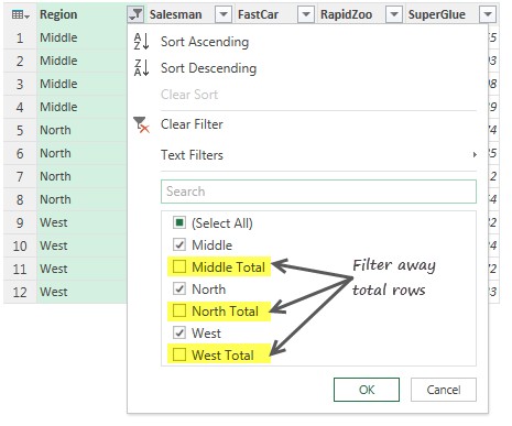
Step 5: Remove sub-total rows by filtering them away

Click on the filter button next to region and filter away all the sub-total columns too. We don’t need them for unpivoting.

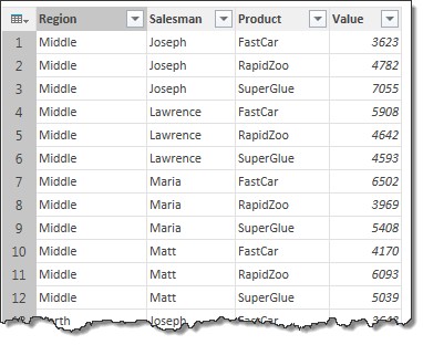
Step 6: Unpivot the data

Now that our data is in correct shape, let’s unpivot.

Select the last 3 columns and click on Unpivot columns button in Transform ribbon.

And we get the unpivoted data.

You can load this data to Excel or to your data model for further processing.

Download example Power Query workbook

Please click here to download the example workbook for this tutorial. To examine the query settings and power query steps,

Open the workbook
Go to Power Query ribbon (or Data ribbon in Excel 2016) and click on Workbook Queries Show Pane option.
Right click on “Unpivot Data” query and choose edit
This opens the query editor. You can examine the steps in the query steps pane to right.

Learn more about Power Query / Get & Transform data:

Power Query (or less intimidating Get & Transform data in Excel 2016) is an impressive technology to help you deal with common data problems easily. If you are an analyst who relies on Excel, learning Power Query is going to make you super productive. Check out below tutorials to get started with this amazing feature.