Here is a fairly annoying problem.
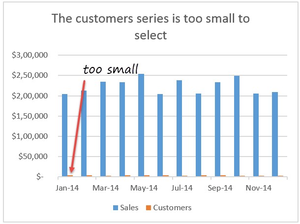
Imagine a chart showing both sales & customer data. Sales numbers are large and customer numbers are small. So when you make a chart with both of these, it looks something like below.
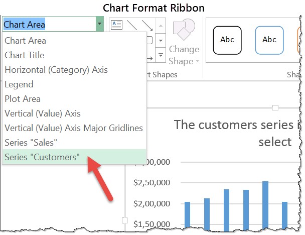
Now, usually to select the smaller, unreachable series, the steps I follow are,
- Select the chart
- Go to Chart Format ribbon and select the series name (as shown below)
But this is a long process with significant click tax.
Here is a simpler alternative. Use arrow keys to select the series you want.
Here is how it works:
- Select one the taller, more prominent series
- Press either up or down arrow keys few times to select the smaller series
- Done!
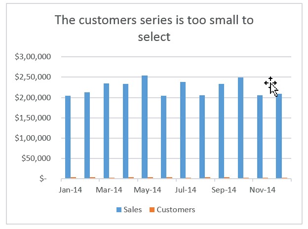
A quick demo of this feature.
So go ahead and use ’em arrow keys to select & format any element in your chart.
Bonus tip: How to know which arrow key to press?
- After selecting the taller series, look at formula bar.
- It should read something like this:
=SERIES(Sheet1!$B$5,Sheet1!$A$6:$A$17,Sheet1!$B$6:$B$17,1) - Notice the last parameter.
- If it is 1, that means the other series is 2 (or 3 …). So you press UP arrow to increment.
- If it is 2 (or 3…), that means the other series is 1. So you press DOWN arrow to decrement.
Bonus Bonus Tip: How to select any individual data points in the series?
Use LEFT or RIGHT arrow keys to select individual data points in a series. This is an easy way to add data labels or change color of one particular data point.
How do you select unreachable chart elements?
I admit. I have been using the chart format ribbon to select unreachable items until today. But once I realized that we can use arrow keys, I feel empowered. While I am not a keyboard shortcut fanatic, I do believe that if there is a faster way to do something with keyboard alone, we should embrace it.
What about you? How do you select chart items? Please share your tips in the comment section.
More tips: on formatting charts, on keyboard shortcuts and quick Excel tips.


