Most advanced Excel users know that slicers are cool. Today, let’s learn how to use slicers to create an awesome selection mechanism for your dashboards and forms.
First see a quick demo
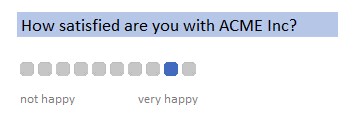
Looks slick, eh? Read on.
Slicers as selection mechanism – step by step tutorial
Just follow below steps to create your own slicer selection tool.
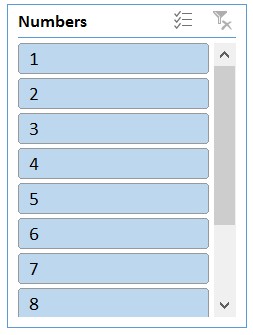
- Enter running numbers (say 1 to 10) in a range, with the header numbers
- Select the range and create a pivot table from it.
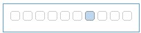
- Select numbers from field list and add it as a slicer. We get this.
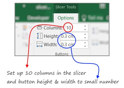
- Select the slicer, go to Options ribbon and set up,
- Slicer columns as 10
- Height & width as small numbers (0.3 cm or 0.1 inch)
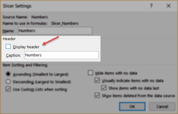
- Disable slicer header. Right click on the slicer and go to slicer settings. Uncheck Display Header option.
- At this stage, your slicer selection tool is almost ready. I say almost because it will still have a border and default style.
- Duplicate any of the slicer styles and set up your own style by disabling slicer border and changing the colors. And your slicer selection tool is ready.
Download the example workbook
Click here to download the slicer selection example workbook. Examine the settings and styles. Play with it to learn more.
Slicer like a ninja, check out below tutorials
Slicers are a must have in any advanced Excel user’s tool kit. Check out below tutorials to learn awesome ways to use them.
- A very comprehensive introduction to slicers
- Using slicer as scenario manager
- Slicer in play – tax burden over the years
- Slicers in play – narrating story of change
- Slicers in play – dynamic dashboard in Excel
Share your slicer inspiration…
Ever since learning about slicers in Excel 2010, I have been using them in all my dashboards and training programs. I like the simplicity and possibilities they offer.
What about you? How do you use slicers in your line of work? Please share your proudest slicer moments, tips and tricks in the comments section.


