Find and Highlight all blank cells in your data [Excel tips] -

True story:

On Friday (17th April – 2015), I flew from Vizag (my town) to Hyderabad so that I can catch a flight to San Francisco to attend a conference. As I had 10 hours of overlay between the flights in Hyderabad, I checked in to a lounge area so that I can watch some sports, eat food while pretending to do work on my laptop. There was a gentleman sitting in adjacent space doing some work in Excel. As I began to compose few emails, the gentleman in next sitting space asked me what I do for living. Our conversation went like this.

Me: I run a software company
He: Oh, so you must be good with computers
Me: smiles and cringes at the stereotyping
He: What is the formula to select all the blank cells in my Excel data and highlight them in Yellow color

Mind you, he had no idea that I work in Excel. We were 2 random guys in airport lounge watching sports and eating miserable food.

Me: Well, what are you trying to do?
He: You see, I am auditing this data. I need to locate all the blank rows and set them in different color so that my staff can fill up missing information. Right now, I am selecting one row at a time and filling the colors. Is there a one step solution to this problem?

Needless to say, I showed him how to do it faster, which led to an interesting 3 hours at the lounge.

End of true story.

So today, let’s understand how to find & highlight all the blank cells in the data.

Let’s take a look at the data:

Here is a sample of data.

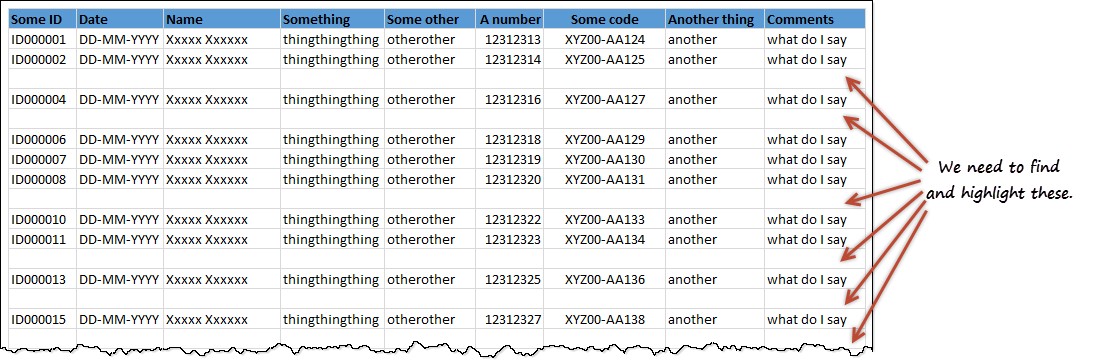
One important thing to keep in mind:

This data is not structured as table.

There are 3 powerful & simple methods to find & highlight blank cells.

Method 1: Selection & Highlight approach

In this method, we just select all the blank cells in one go and fill them with yellow color.

First select the entire range of cells where you data is located. Using CTRL+Arrow keys is not going to work because of the blank cells in-between. Instead, follow this:

Select the top-left cell of your data (say B2)
Click and drag the little rectangular box in vertical-scrollbar all the way down.
Hold Shift and click on the very last cell (bottom-right)

Now that all the data is selected,

Press F5 and click on Special
Choose blanks. Click ok.
This will select only the blank cells.
Fill yellow (or other) color by clicking the fill icon and selecting the color
Done!

Here is a quick demo of this:

Method 2: Filter approach

The above approach (selection & highlight) works fine if you care about blank cells anywhere. What if you just want to find & highlight only rows have blanks in a certain column. Say, you want to highlight all rows where comments are empty.

In this case,

Select all data using the steps in method 1.
Press CTRL+Shift+L to activate filters
Keep the selection on & Filter the column you want to show only blank values
Now fill yellow color
Done!

Method 3: Conditional formatting approach

Both method 1 & method 2 have a draw back. If your data changes, you must clean up & highlight again.

This is where conditional formatting shines. You can tell Excel to highlight cells only if they are blank. Once some data is typed in (or copy pasted or connection refreshed), the color will go away automatically.

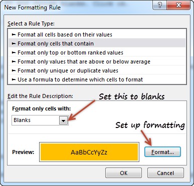
To set up conditional formatting,

Select all the data
Go to Home > Conditional Formatting > New rule
Click on “Format only cells that contain”
Change “Cell Value” option to “Blanks”
Set up formatting you want by clicking on Formatting button
Click ok and you are done!

This will automatically highlight all blank cells in your favorite color.

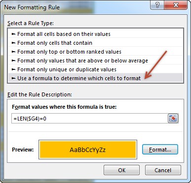
Oh wait, what if I want to highlight entire row if a certain column is blank?

You can use conditional formatting in such cases too. Follow these steps.

Assuming you want to check for blanks in Column G and your first data point is in G4.

Select all the data (just data, no headers)
Go to Home > Conditional Formatting > New rule
Select rule type as “Use a formula…”
Type the formula as =LEN($G4)=0
Set up formatting you want
Click ok and you are done.

Wait a sec, What is the `LEN($G4)=0` thing?

LEN() formula tells us what is the length of a cell’s content. So if a cell is blank, LEN(cell) would be 0.

$G4 is a mixed reference style. This way, even when conditional formatting is checking other columns, it still looks in column G to see if that is really empty.

Bonus tips:

Q) How to highlight if either of column G or H are blank?
A) =OR(LEN($G4)=0, LEN($H4)=0)

Q) How to highlight if both column G & H are blank?
A) =AND(LEN($G4)=0, LEN($H4)=0)

Go ahead and whack them blank cells.

How do you deal with blank cells?

Do you sneak up on an unsuspecting fellow passenger in an airport lounge and ask them how to deal with the blank problem? Do you manually select the blank cells and deal with them one at a time? Or do you use some ninja level trickery to fix the blanks?

Go ahead and tell me your blank story in the comments.

Fill the blanks in your Excel knowledge

If you have gaps in your Excel know-how, then you have come to right place. Use below links and fill those blanks.

direct tag