How to add a lot of Goal Seeking to a model -

Recently in the Chandoo.org Forums, MR06 asked the question, “I am trying to create a sensitivity table that tells me what amount of equity I need to include in a deal in order to get a fixed IRR as the year 3 sales price changes.”

MR06 was using Goal Seek to change the equity input so that the IRR achieved 25% value. But he wanted to do that for a number of Year 3 price changes in the model.

He could obviously change the Year 3 value manually, then run a Goal Seek and write down the Solution and repeat for the range of Year 3 prices changes.

Or he could have setup a macro to do the same and tabulate the results.

Eventually I provided a solution which uses a Data Table and some formulas to determine these values

This post will examine the technique used to solve the problem for MR06

The Problem

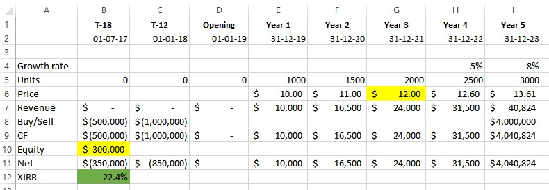
This is MR06’s model. It is a simple financial model of an investment in some units over a 6 1/2 year period.

The problem is that MR06 wants to know what Equity value B10 is required to achieve an Internal Rate of Return (IRR) of 25% subject to varying the Year 3 Price, cell G6.

Goal Seek

This problem can be solved using Goal Seek
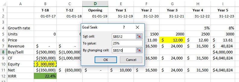
Goto the Data, What-If-Analysis, Goal Seek Tab

Set the dialogs in the Goal Seek to the values shown above and press Ok

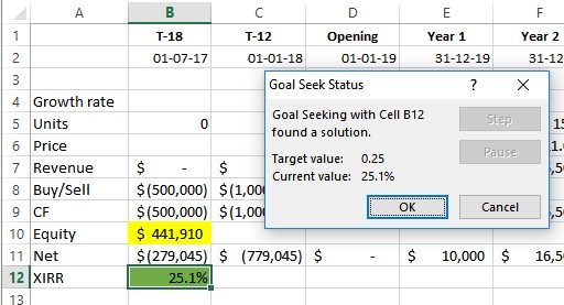
Excel sets the value in cell B12 to the value of $441,910 and shows an IRR of 25.1%. This small discrepancy will be discussed later.

MR06 can now manually repeat that changing the values of G6 between each iteration. Except that MR06 has many many models and wants to do that for variations in the Year 3 Price from $8 to $15.

Data Tables

An alternative method to solve this is to use a Data Table to feed in the starting values for both the Year 3 Price G6, as well as a list of Values for the Equity Contribution B12.

The Data Table will then retrieve a list of the IRR’s for the various combinations.

Then we can then setup a formula to calculate the Equity contribution required to achieve the target IRR value of 25%

You can follow along with a copy of the worked example: Download Example File Here

Firstly setup a Data Table

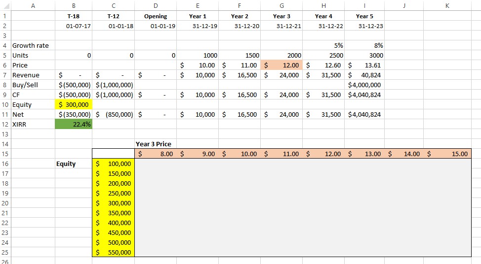
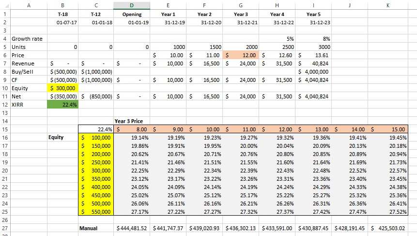
Setup a list of required Prices for Year 3 in a Row D15:K15 and a list of possible Equities in a Column C16:C25

I have colored the cells to simplify which cells are linked to which parts of the Data Table.

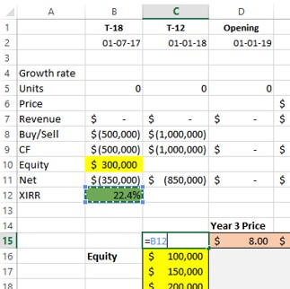
In the Top Left cell C15 link that to the Target IRR cell using =B12

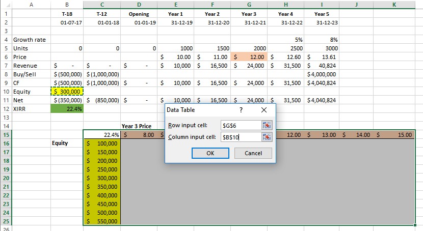
Now select the whole area C15:K25 and goto the Data, What-If-Analysis, Data Table Tab

Complete the Data Table dialog
Row Input cell: $G$6
Row Input cell: $B$10

Press Ok

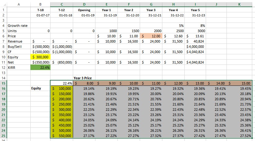
Excel will now fill in the Data Table area with the IRR’s from the combination of Each Row (Equity) and Column (Year 3 Price)

At this point we now have a table of IRR’s from the combination of Each Row (Equity) and Column (Year 3 Price), but we can see that we don’t have an actual solution, only approximate solutions for each Year 3 Price.

Our goal was to find the Equity value which returned a 25% IRR

We can use the Excel Forecast() function to interpolate the exact answers based on the data in the Data Table

Forecast allows us to forecast a Y value based on an X value from a Table of Known X and Y values
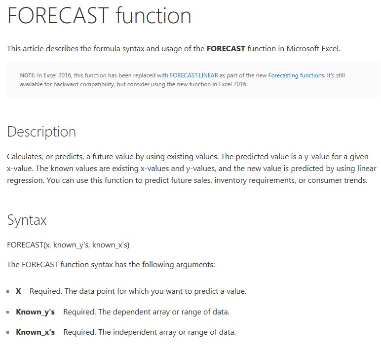
You can read the excel help about forecast

We can see from the help that Forecast uses the syntax:
=FORECAST(x, known_y’s, known_x’s)
In our example we are seeking a known value of the IRR of 25%
We have a List of Known X’s which is the IRR’s in the Data Table and the list of known Y’s is the corresponding list of Equities in Column C

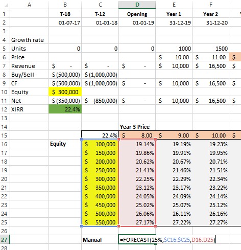
To test this in cell D27 type the following: =FORECAST(25%,$C16:$C25,D16:D25) and press Enter
Excel will return $444,481.25

This is the equity required to return 25% IRR based on a Year 3 Price of $8.00

You can copy Cell D27 across and you will now have a Table of all the equities required for all Year 3 Prices.

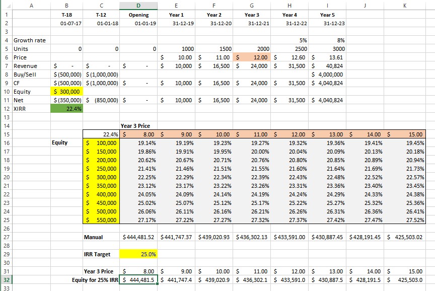
A neater solution is to also allow the IRR to be set as a variable. This way it can be changed and the new equities automatically shown for each Year 3 Price change
In Cell D29 type 25%
Then setup a Row of Year 3 Prices in cell D31 type: =D15
Copy D31 across to K1
Then in D32 type: =FORECAST($D$29,$C16:$C25,D16:D25)
Copy it across to K32

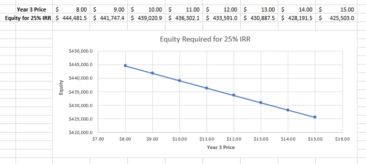
You now have a table of Year 3 Prices and the required Equities to achieve a 25% IRR

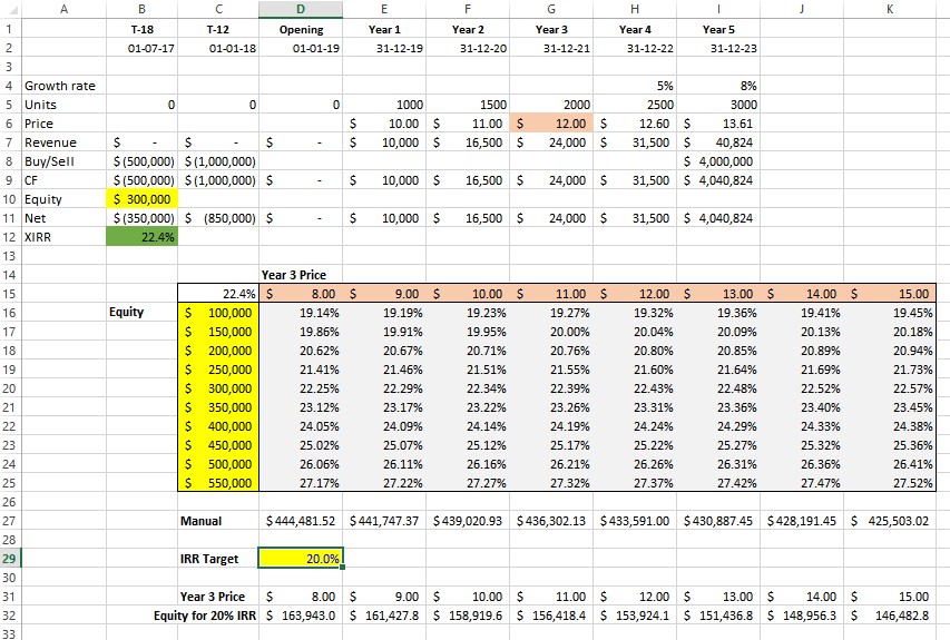
You can simply change the Required IRR in Cell D29 eg 20%
And you will have a Table of the required Equities to achieve a 20% IRR

The good thing about having this as a separate table is that it can easily be graphed
Select the Table and got the Insert, Chart Tab
Select an appropriate chart type

One warning

In this example the model appears to be very linear, this means there is a direct or straight line relationship between the Equity and the IRR for a given Year 3 Price

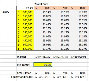
If we choose a value of equity of say 30% we can see that we need an equity of $725,020 for a Year 3 Price of 8.00

It is important to note that the value of $725,020 is outside the range of the Equity values we set in Column C

In this case we should check that this is still a valid Forecast

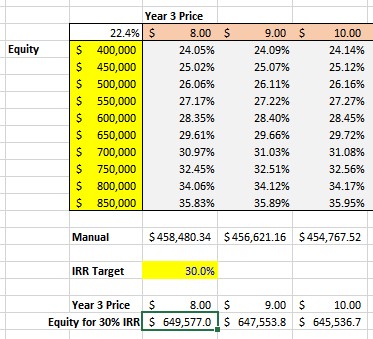
To do this reset the Equity values in Column C to that shown below, ensuring that the equity values extend both below and above the expected equity value we saw of $725,020

We can now see that the Equity value required is $649,577.

Warning:

Those who are observant will notice that the Equity value of 649,577 should have an IRR of slightly less than 29.61%, not 30%

This is because although the model appears linear, it is in fact not exactly linear.

The model’s non-linearity occurs for a number of reasons but primarily is that XIRR is not an exact function. It is an Iterative Function and to quote from Microsoft Help “Excel uses an iterative technique for calculating XIRR. Using a changing rate (starting with guess), XIRR cycles through the calculation until the result is accurate within 0.000001 percent.”

For all intention purposes it is close enough to linear that we don’t notice the differences.

If it was perfectly linear the extrapolation to 30% which was outside the original Equity range would have given us the same result of $649,577 not the $725,020 that it returned. Non-linearity is magnified once the extrapolation used in the Forecast Function is outside the range of the known Y values and we need to always check for this.

This non-linearity causes small discrepancies in the Excel functions like IRR and Forecast, of which we are using both.

Forecast uses a least squares approximation to best estimate a line of best fit, but it is just that, an approximation.

If you are wondering how close the model is to being linear, it is 99.77% fit to being linear

This is calculated using the r value or Pearson() function
D50: =PEARSON(C16:C25,D16:D25)
=0.997747518
That is the closer the value is to 1 the more linear it is.